The electricity grid functions in a real-time environment where the demand must be met by supply at all time. With the increased adaptation of renewable resources, it is more important than ever to balance the power grid and avoid any power shortages. This project is an interactive and visual representation of control strategies used to solve the energy arbitrage problem.
This project has been my capstone project as a 4th year Sustainable and Renewable Energy Engineering student
at Carleton Univerity. With the education Carleton Univerity has provided, I was able to gain a deep understanding
in energy engineering and build this project.
I'm immensely grateful to Dr. Mostafa Farrokhabadi and Prof. Shichao Liu for mentoring me throughout this project.
The idea is simple, power grid functions like the real-time market.
The price of power depends on the balance of supply and demand.
If the demand is low, the price of power drops, shifting the power production to lower-cost resources, such as wind, solar, hydro or nuclear.
When the demand is high, the grid operator either spins up less efficient generators or buy power from other
operators to compensate for the demand causing the price of power to increase.
The increased penetration of renewables is causing unpredictability in power generation which conveys an unstable
grid and swinging electricity prices. With the help of large energy storage solutions, these problems can be overcome
allowing for a larger renewable presence. One of the more favored energy storage solutions is grid integrated batteries
due to their fast response time. Assuming the existence of the grid integrated batteries, with the historic hourly electricity data,
an algorithm is needed to decide to buy, sell or hold power in a given time. Finding an optimal solution becomes especially challenging
due to the unpredictability of the price of power. The purpose of this project is to compare various algorithms
and strategies to find the optimal control strategy.
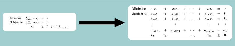
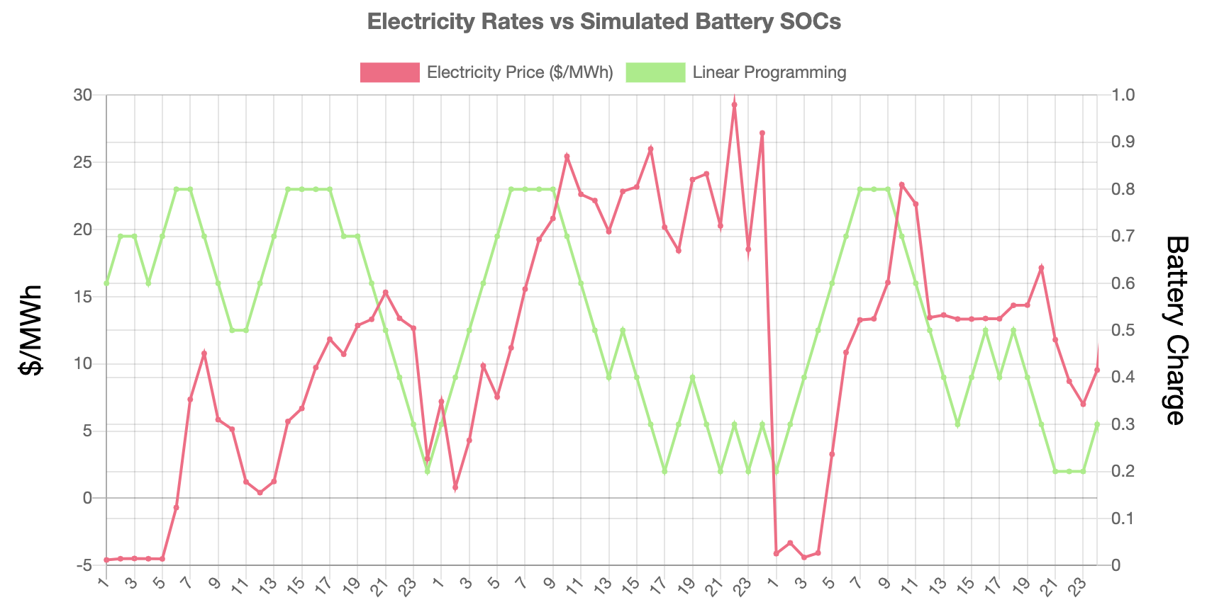
LP is a methodology used to find a global optimum in a linearly defined space. Which in this case, assuming the price of power is known for a defined period, it is possible to find the optimal charging strategy. Thus, the maximum amount of reward or money that can be made is determined by this optimal solution. In a real-world scenario, it is impossible to predict the feature perfectly. However, it can be used as a benchmark to compare the performances of other control strategies.
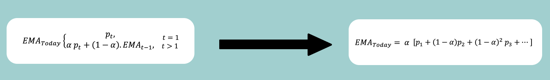
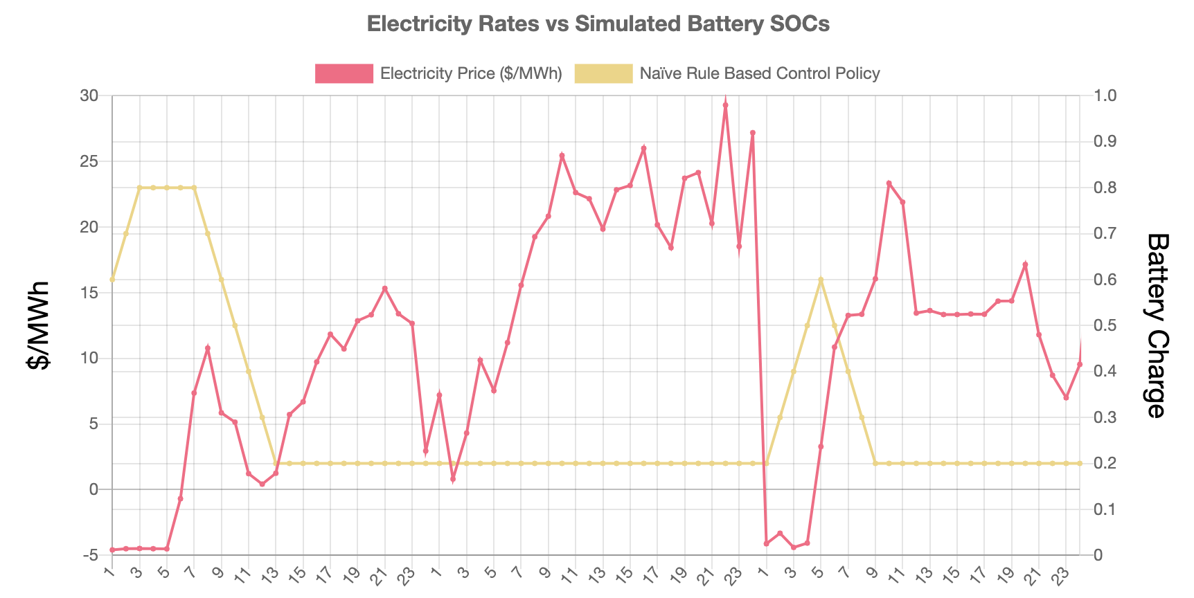
Naïve Rule Based Control Policy uses the Exponential Mean Average (EMA), which is a type of mean average calculation with the difference of, placing a larger weight on the most recent data points. Compared to linear programming, this strategy does not require to hold knowledge on the feature. It requires a limited number of past observations to determine if the current price is higher or lower than the average. When the price dips below the EMA and the battery is below the max SOC, it starts charging, and the other way around. Although it sounds simple, this strategy is widely used by day-traders.
Reinforcement Learning is not a new concept; however, it became famous after DeepMind team published a groundbreaking paper called ‘Human-Level Control Through Deep Reinforcement Learning’ in 2015. They found a solution to successfully coupled neural networks with reinforcement learning and achieve human-level control in Atari games.
DQL consists of an agent (actor) and an environment. The agent intakes observations from the environment evaluate its’ current polity and return the best possible action. This action produces a new state and reward, by the environment. This cycle continues until the end of the episode. The goal of the agent is to maximize the reward received at each episode.
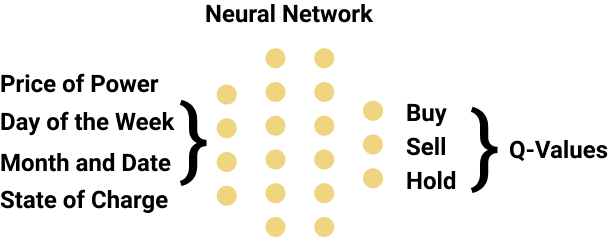
In this project, the state variables are set as the current price-of-power, time, month and the state-of-charge. The agents’ action space is limited to buying, selling or stalling electricity. Considering the size of the environment and the need to evaluate unseen states, a differentiable policy is needed. Thus, a fully connected two-layer neural network was used as the policy network. The word “deep” in DQN comes from the existence of deep learning.
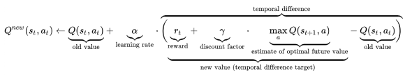
Deep Q-Learning is a model-free reinforcement learning technique meaning, the agent does not require a predefined knowledge of the environment. To optimize its policy, DQL uses experience replay and Temporal Difference (TD) error, taking advantage of the episodic environment.

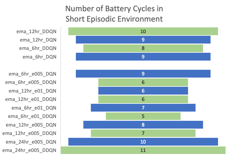
Using a grid search method, 36 agents were trained to determine the impact of the hyperparameters on the optimal policy. Three major environment strategies were set and the influence on the final optimal strategy can be seen. Also, for each DQN and DDQN strategy three episode lengths, (24-48)hr, (48-100)hr and (100-200)hr were tested.
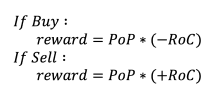
The reward function is simple, the amount of power bought (-) or sold (+) multiplied by the current price.
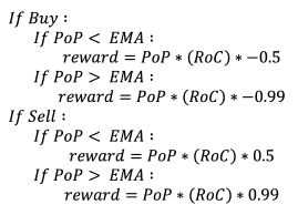
The reward function includes a coefficient determined by EMA. This coefficient rewards the agent if the power bought below average or sold over the average price.
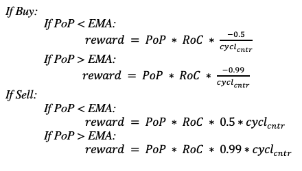
The reward function includes a coefficient determined by the combination of EMA and the cycle decay. The cycle decay was modelled by a negative exponential function. With each taken action, the battery cycle was counted, and the cycle decay was determined and added to the reward coefficient.
The test dataset is large to find the optimal solution, however,
it was estimated to be 14219.91 $ with 10^-5 tolerance.
To obtain this value, the battery cycle count was calculated to be 81.
For the mean calculation, four window sizes were tested, ranging from 6hr to 48hr. By using a window size of 6hrs, the reward was calculated to be 3100.88$ with 23 cycles. Increased window size (48hr) resulted in a slightly better return of 3184.32$ , reaching the limit with the same cycle count.
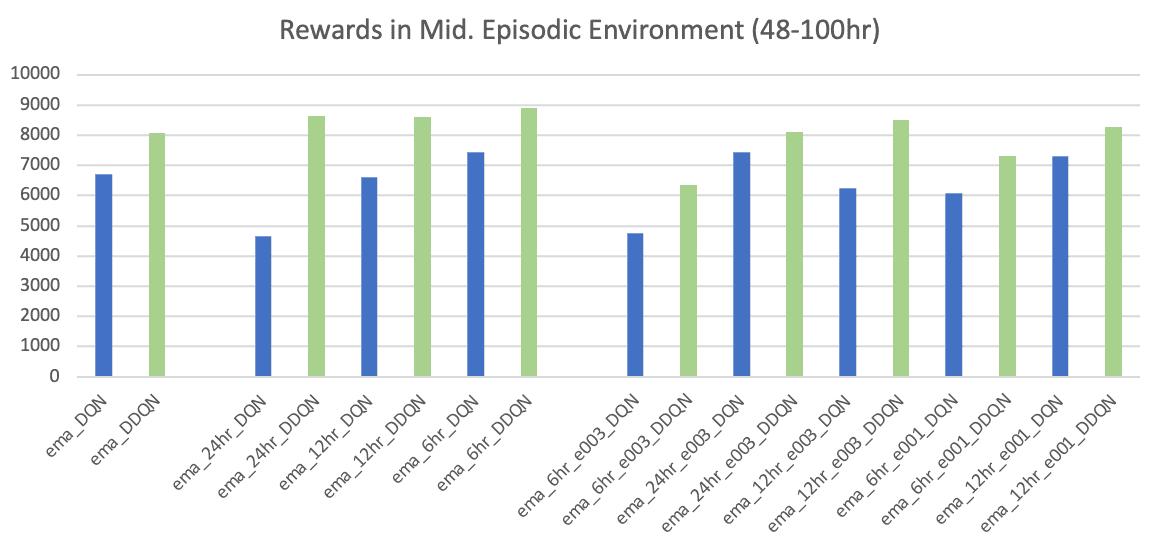
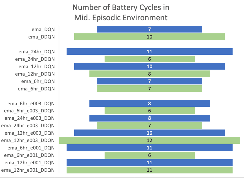
The agents trained using the 1st strategy returned a similar total reward in the medium and long sequences. DDQN trained in the mid-range produced a slightly more reward, toping 8064.00$ with 10 battery-cycle count . This result indicates that deep reinforcement learning produced a 2.5x greater return then the Naïve Rule Based Control Policy.
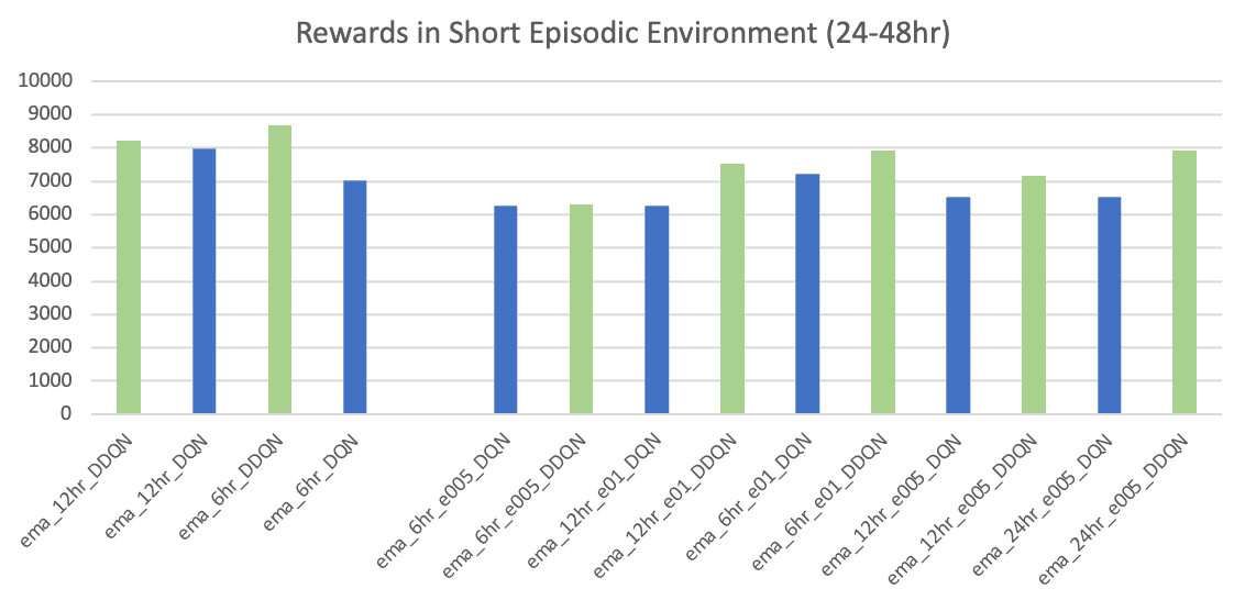
While analysing the results using the test set, models trained with the 2nd and 3rd strategies’ rewards were also calculated using the 1st strategy.
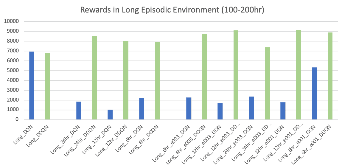
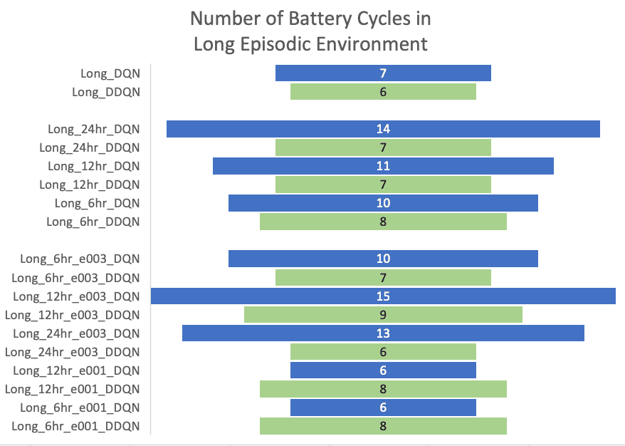
Following the 2nd and 3rd strategies, although the DQN and DDQN performances on short episodes are not distinctive, DQN agents trained in the longer episodes produced a significant performance drop. With the increased episode lengths, DQN became unstable and suffered from maximization bias. The DDQN architecture overcame this challenge producing significantly improved outcomes with a much stable strategy. The DDQN agent trained using the 3rd strategy in long episodes returned the maximum reward of 9136.00$ with only 8 cycles .